Google Sheets Autofill Number to Repeat Not Continue

Multiple Ways of Serial Numbering in Google Sheets

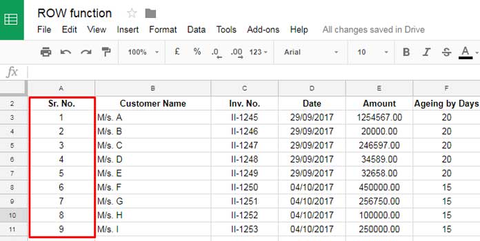
As you may know, a standard format starts with a serial number column. To more precise it will be like serial number, description, client name, etc. Under the serial number column, you can number rows in different ways. Here we can learn about auto serial numbering in Google Sheets.

There are multiple ways one can adopt to put the serial number in Google Sheets. Before going to tell you how to auto number rows in Google Sheets in dynamic ways, I should tell you other available options that may be useful for beginners.

At the end of the post, I have also shared the information on how to auto-increment alphabets as well as Roman Numerals in Google Sheets.

So let us begin with different auto serial numbering in Google Spreadsheet.

Auto Serial Numbering Using Simple Formula

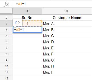
In the above example, our serial numbering starts from row A3. Here in this case, in Cell A4 use the formula =A3+1 and then copy and paste this formula to the cells down. See the above screenshot.

This is commonly using the numbering method in Google or Excel spreadsheets. It can auto-adjust rows numbering when insert or delete rows in between.

Auto Row Numbering Using the Fill Handle

Unlike Excel, Google Sheets fill handling behaves differently. You can't use the fill handle to auto-fill the number in Google Sheets this way. It works perfectly in Excel. The below screenshot is applicable only in Excel.

Update: Now it works in Google Sheets too!

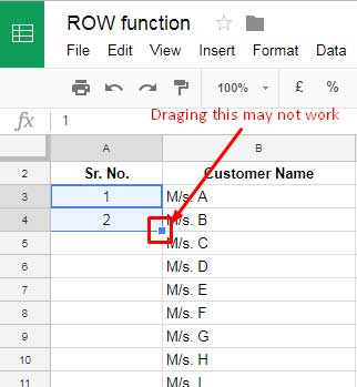
serial numbering using fill handle in Google Sheets

Here what you want to do is manually enter the first two serial numbers and then drag the fill handle to down or double click on the fill handle.

Automatically Put Serial Number in Google Sheets Using the Row Function

Here I've used the ROW function. This function can return the row number of a specified cell.

Syntax:

          ROW([cell_reference])

Example:

          =row(A3)

Output=3

          =row()

This formula will return the row number of the formula applied cell. Now back to our topic.

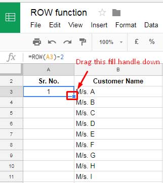
As per the example (refer to screenshot above) our row numbering to be started from row number 3.

The row number function applied in Cell A3 is ROW(A3). It will return the row number 3 in the active cell. But we need our serial number to start from 1. So I have used the formula below.

          =row(A3)-2

Then you can either copy and paste the formula to down or drag the fill handle down. When you delete any row in between, in this case also, the serial number will automatically get adjusted.

Note: If you want to have the serial numbers to get change when the data group changes see this tutorial – Group Wise Serial Numbering in Google Sheets.

Dynamic Auto Serial Numbering in Google Sheets

The ultimate way of auto serial numbering in Google Sheets!

This is the best option to automatically fill the serial number in Google Sheets. Here we can use a kind of formula which is a combination of IF, ArrayFormula and ROW function.

First, see the below formula in Cell A3. It's as per our sample screenshots above.

          =ArrayFormula(if(B3:B<>"",row(A3:A)-2,""))

I will explain to you how this formula works and how you can use it in your Spreadsheets.

As per the above example, you just want to apply the formula in Cell A3. No need to copy and paste it down. It will automatically do the numbering to the cells down. How?

Details (Formula Explanation)

The formula row(A3) returns the cell number in A3, i.e. the number 3. We can use a -2 to make it 1. When you want to use infinitive rows you should use this formula as row(A3:A)-2 and also include the ArrayFormula function.
When you want to auto-fill serial numbers, you should know how to limit the numbering to a specific number of cells. We did it by using the IF logical function in Google sheets here.

We have customer name under column B. If column B has no value, then the above formula won't put any number to the corresponding cell under Column A.

Now the array function. Without the array formula, we can't automatically expand the formula to the below cells.

Now how to use this formula for your needs and that is important. See a few more formulas below.

When you want your serial number to start from Column H2 and your rest of the data on the right side. Use this formula in cell H2.

          =ArrayFormula(if(I2:I<>"",row(H2:H)-1,""))

Now another formula in cell J3.

          =ArrayFormula(if(K3:K<>"",row(J3:J)-2,""))

Here the serial numbering will start from cell J3. You can use the above formula to automatically fill serial numbers in any column. Just change the cell reference in the formula as per your data.

Conclusion

Please note that ROW is not the only function to populate serial numbers in Google Sheets. There is a relatively new function called SEQUENCE. You can read more about this function here – How to Use Sequence Function in Google Sheets.

Although generating auto serial numbers using the Sequence function is simple, the majority of Sheets' users depend on the ROW function. It's so much popular.

Lardner Margance